1. Introduction
The main purpose of this paper is to assess the cost efficiency of Banco Ciudad de Buenos Aires’s (BCBA) bank branches using a Stochastic Frontier Analysis (SFA). Likewise, we use efficiency measures to gauge new branches. We estimate cost efficiency and then compare the cost efficiency of the worst situated branches with the best performers according to the cost efficiency criteria. This is one of several possible uses of the tool. Many other possible managerial recommendations can be developed.
The BCBA is the official bank of Buenos Aires City. It was founded in 1878 and ranks as the eighth largest provider of bank loans in Argentina and the second local one in the mortgages market. It has 66 branches and some 3,200 employees. Nowadays, one of the bank’s goals is to move beyond the boundaries of its historical area of influence (Buenos Aires City and suburbs). As a public bank, this goal faces some management constraints (for instance, it is not a pure profit maximizer, and employees enjoy stability as public servants), plus regulations of the Central Bank of Argentina restrict decisions to all banks in the country concerning free branches’ creation or closing.
At management level, the BCBA currently uses two methods to analyze branch performance. The first is a system of quarterly and annual targets, determined by business volume and the complexity of each branch. Targets are set for “strategic products and services”, such as loans, new current account and savings account openings, the number of desk and cashier operations, insurance policies sold, and so on. Targets are summarized in an output index by assigning weights to each individual goal and by dividing the weighted output average by its maximum. The second method is a partial productivity ratio set, computed over a set of performance indicators such as loans per employee, loans per branch, or customers per employee.
More comprehensive and exhaustive measures to assess efficiency and to compare relative performance are frontier studies. Two strands of the latter are mathematical programming models (mainly using Data Envelopment Analysis - DEA) and econometric models (mainly using Stochastic Frontier Analysis - SFA). This study employs the SFA technique. Each method has comparative advantages and disadvantages against the other; SFA is a preferred method when estimating cost efficiency (our goal), and DEA is customarily used when the purpose is to estimate technical efficiency (Coelli, Rao, O'Donnell & Battese, 2005).
We use SFA for estimating cost efficiency, not technical efficiency. In the latter case the multiple output criteria cannot be applied (for instance, when estimating a production frontier y = f(x1, x2, …, xn) where xi from 1 to n are inputs and y is the (only) output1. Nevertheless, we are estimating a cost frontier C=(y1, y2, …, yn, w1, w2, …, wn-1) where C is used for denoting costs, yi from 1 to n are the different outputs and wi from 1 to n-1 are the relative prices of the different inputs relative to the n-th input (the numeraire). Thus, the cost function allows to estimate cost efficiency in a multiple-output environment.
With respect to strengths and weaknesses of SFA against DEA, there are relative advantages of the second method to address multi-output technical efficiency computing, the possibility of working with small samples, the sensitivity of the method to outliers -which allows the investigator to discover errors in the database-, and the absence of constraining to a particular and probably arbitrary functional form. On the other hand, SFA allows statistical significance tests, permits multi-output estimates -in the case of cost functions-, SFA yields a function which describes the behavior of the bank, under some economic objective (such as cost minimization or profit maximization), and SFA allows to separate inefficiency from statistical noise (at the cost of making some hypothesis on the statistical distribution of the inefficiency component).
In frontier models, a numeric value is assigned to the efficiency of each branch which makes it possible to identify both the over-utilization of inputs - or the under-production of outputs - and best practices. SFA models can supplement more commonly used managerial indicators (mainly accountancy ratios) to determine inefficiency and help to provide remedies.
Identifying a branch’s relative performance is a starting point in a comprehensive evaluation of some branch network efficiency. The efficiency scores allow building a performance ranking by identifying the worst and best performers, detecting for remedial action, for incentive design, or for the reallocation of resources. In the same vein, high-performing branches may serve as instructive role models for low-performing ones (Pastor, Knox & Tulkens, 2003). Or, at least, given binding constraints on management, or regulations that prevent the exploitation of all the results potential2, new branches could be designed with the attributes of the best performers, which is the criterion followed in this exploratory study.
The structure of the paper is the following: after this introduction, section 2 presents the literature review. Section 3 summarizes the method. Section 4 describes the database. Section 5 presents the results and the managerial implications, and section 6 discusses them. Lastly, section 7 concludes.
2. Literature review
According to Hughes and Mester (2008), there are two broad approaches to measure banking efficiency and thus to explain nonstructural and structural performance. The former uses a variety of financial ratios or the market value of the firm, capturing aspects of performance to compare banks. The structural approach relies on the theoretical models of the bank’s technology and on the assumption of some objective-function optimization goals. The studies assume that the banks choose a production plan that minimizes costs given their output mix and input prices or that they maximize profits given input prices and outputs.
It is difficult to estimate banking efficiency because of the variety of services commercial banks offer. Following Stavárek (2005), three main approaches in the literature define the input-output relationship in financial institutions.
First, the production approach considers banks as producers of accounts and loans, defining output as the number of such accounts and loans. This method defines inputs as the number of employees and capital expenses in fixed assets. The approach centers on operative costs and ignores interests paid. Second, the intermediation approach originates in the traditional role of banks in transferring financial resources from savings suppliers to savings demanders. Operative and interest costs are the most important inputs contemplated here, while the main outputs are interest income for credits and investments and charges for services. Third, the assets approach highlights the role of financial entities as credit originators. This view is a variant of the intermediation approach, differing in the outputs than the latter approach.
None of the three approaches can fully capture the dual role of financial entities as providers of transaction services and conveyors of savings from suppliers to demanders. Nevertheless, there is a reasonable consensus in the literature about the banks’ inputs and outputs. Loans and other relevant assets should be considered outputs according to intermediation and asset approaches. Some controversy exists over the role of deposits. There is an empirical test to determine whether deposits act as an input or output. Let us call variable costs (VC) and deposit levels (x). If deposits are an input, then ∂VC/∂x<0, thus, increasing the use of some input should decrease the expenditure in others. Instead, if x is an output, it is expected that ∂VC/∂x> 0. Thus, output can be increased only if input expenditures are increased (Hughes & Mester, 2008).
Inputs and outputs are flows. When data on input flows are not available, stocks are used as proxies. A third input, beyond labor and capital, are the flows of financial services, which are hard to measure with the data that are normally available. Thus, they are approximated by stocks, such as loans and deposits (López, Appennini & Rossi, 2002).
Berger and Humphrey (1997) encourage the efficiency research at branch level after presenting a survey of empirical literature of branch and bank system efficiency. They observe that the literature at bank branch level was, at the time of their survey, still limited by comparison to bank system efficiency measurement.
Firstly, we describe the literature on branch efficiency after the seminal survey of Berger and Humphrey (1997), and secondly, we summarize the findings and their importance for this study. The literature related to banking system efficiency, by opposition to bank branches efficiency, continues to be more extensive. For a very recent and exhaustive discussion of the former literature, see Asimakopoulos, Chortareas and Xanthopoulos (2018).
Athanassopoulos, Sotiriou and Zenios (1997) analyze the efficiency of bank branches networks in different countries (the United Kingdom, Greece and Cyprus), suggesting guidelines for branch efficiency improvement.
In turn, Berger, Leusner and Mingo (1997), measure the efficiency of a branch network over a large American bank. They find evidence of severe “over-branching”. The X-inefficiencies they find exceeded 20% of operating expenditures.
Camanho and Dyson (1999) assess the performance of Portuguese bank branches. The analysis focused on the relation between branch size and performance.
Zenios, Zenios, Agathocleous and Soteriou (1999) develop a study commissioned by the Bank of Cyprus, with the objective of set benchmarks of performance and to address the effects of a cyclical component of the demand due to tourism. The analysis revealed branch resource underutilization during the low season.
Athanassopoulos and Giokas (2000) present an application of frontiers for the Commercial Bank of Greece. They derived lessons for managerial utilization in aspects such as input/outputs sets, and incentives concerned with managerial control systems.
Kantor and Maital (1999) build a method to measure product-specific inefficiency in bank branches for facilitating a precise measurement of waste, and identify its causes. The model measures inefficiency both for customer services and transactions in a Middle Eastern bank. The results are useful for managers since they yield quantitative performance indicators useful for their activity.
In Donatos and Giokas (2008), efficiency models were applied to a sample of branches belonging to a Greek Bank, in order to discuss differences in the results with respect to accounting the ratios customarily used. The study highlights the relative superiority of the structural efficiency estimating methods.
According to Chaffai and Dietsch (2009), environmental variables (concerning the macroeconomic landscape, industrial organization and regulatory environment) are useful both at studying bank system and branch networks’ efficiency, because they reduce the efficiency gaps among banks and between branches of the same bank.
Potential managerial usages of the results are presented in Yang (2009). Yang (2009) evaluates 240 branches of a large Canadian bank in the greater Toronto area. Special emphasis was placed on how to present the results to management in order to provide them with guidance, along with ways to implement changes.
To measure the relative efficiency and potential improvement capabilities of bank branches by identifying their strengths and weaknesses, Eken and Kale (2011) develop a performance model. Under both production and profitability approaches, efficiency characteristics of branches -grouped by different sizes and regions-, have similar tendencies. Overly small and excessively large branches in the sample needed special attention.
Chang, Chang-Lin, Yu and Chia-Fu (2011) try to identify through an estimated model room for enhancing efficiency in bank branches. In doing so, they generate a variable from the non-performing loan ratio and introduce it in the efficiency model as an undesirable output. They find branches with an excess of staff expenses as well as unprofitable ones. Those results are generally present in the inefficient branches.
Branch efficiency studies are also used to compare performance between state-owned and privately owned banks. Yang and Liu (2012) present frontier efficiency results which indicate the latter are relatively more efficient. In addition, the sensitivity analysis helps bank management to identify branches' efficiency and weaknesses.
Paradi and Zhu (2013) survey 80 bank branches efficiency frontier studies in 24 countries/areas. They discuss key issues related to model design.
Paradi, Min and Yang (2015) examine the operational efficiency of one of Canada’s largest bank branches. They find that efficiency is influenced by staff allocation and the quality of service provided. The study shows the trade-off among pro productivity policies and “best practices”: “full efficiency” is perhaps a more complex concept. For instance, staff under strong pressure for client satisfaction can react, leaving the company and its replacement to increase costs and -in the phase of training- can harm customer service.
Hayat, Anggraeni and Bakhtiar (2017) aim to measure relative efficiency and to develop potential improvement tools from their model for Bank Entrepreneurial Financial Group (EFG) Syariah branches for the period 2014 and 2015. They utilize a DEA technique with production and profitability models. Another purpose was to measure productivity change in branches between periods using the Malmquist Index.
Recently, Niaki and Shalmani (2016) have studied the performance of Saman Bank branches in Iran, and ranked them using a stochastic frontier function, input-oriented approach.
Bikker and Bos (2008) present a complete study that compiles and tabulates the results of different bank efficiency studies to that date (where branch efficiency studies are a subset). No study on branch efficiency on Argentine banks has been found, while there are some for the entire local financial system; Guala (2002) being the seminal study in this respect.
In Table 1, we summarize key aspects of the studies we analyze for this literature review section.
Table 1 Summary of the literature review on banking branch efficiency
| Authors | Branches | Period | Place | Inputs, Input Prices and Cost Variables | Outputs | Environmental variables |
|---|---|---|---|---|---|---|
| Athanassopoulos et al. (1997) | 196, 185, 126 | 1994 | United Kingdom, Greece and Cyprus | Labor costs Computer terminals Branch size | Savings accounts Checking accounts Loan accounts Business accounts | Not mentioned |
| Berger, Leusner and Mingo (1997) | 760 | 1989-1991 | United States of America | Average wage Average rental Price of capital Operating costs (both intermediation approach and transaction approach | Consumer accounts Business accounts Different types of transactions | Not mentioned |
| Camanho and Dyson (1999) | 168 | 1996 | Portugal | Employees Floor Space OPEX External ATM | General service transactions performed by staff Transactions in external Automated Telling Machines (ATM) Accounts Value of savings Value of loans | None |
| Zenios et al. (1999) | 145 | 1997 | Cyprus | Managerial personnel Clerical personnel Computers Space Current accounts Saving accounts Foreign currency and commercial accounts Credit applications | Hours of work produced by branch | None |
| Athanassopoulos and Giokas (2000) | 47 | 1988-94 | Greece | Labor hours Branch size Computers Labor costs OPEX Running costs for buildings | Deposit and transfer transactions Credit transactions Saving deposits Current Deposits Demand deposits Time Deposits Total loans Non-interest income | None |
| Kantor and Maital (1999) | 250 | 1999 | Israel | Model 1: Labor costs Services Areas for Services Model 2: Labor costs Transactions Area for transactions | Model 1: Demand deposits accounts Weighted customer service transactions Queue replacing actions. Model 2: Credit cards Weighted transactions Commissions Savings accounts activities | None |
| Portela and Thanassoulis (2007) | 57 | 2005 | Portugal | Staff Rent | Number of transactions Increase in the number of clients Increase in the value of current accounts Increase in the value of other accounts Increase in the value of titles deposited Increase in the value of credit by bank Increase in the value of credit by associates | None |
| Gemmel and Bourgonjon (2002) | 1720 (from a merger of two banks) | NA | Belgium | Several in several models to tests different definitions of efficiency | Several in several models to tests different definitions of efficiency | Non-discretionary input variables |
| Donatos and Giokas (2008) | 240 | 2002 | Greece | Personnel costs Running costs Other operating expenses | Deposit based transactions Loan based transactions Remaining transactions | None |
| Chaffai and Dietsch (2009) | 1618 | 2004 | France | Financial costs (of deposits and from borrowing) Labor costs Non-labor costs | Three measures of bank profits (gross, operative and net) | None |
| Yang (2009) | 240 | 2005 | Canada | Sales (Full Time Equivalent) FTE Service FTE Support FTE Other FTE | Number of transactions (new consumer loans, new interest bearing current accounts, new menu accounts, processing branch deposits to menú accounts, to process withdrawals from menu accounts, to update passbook from menu accounts in branch, to transfer funds in branch) | |
| Chang et al. (2011) | 151 | 2005 | Taiwan | Personnel expenses Interest fees Incidental expenses | Net profit Operating profit Interest gains Total loans Total deposits | Non-discretionary input variables (non performing ratio loan |
| Eken and Kale (2011) | 128 | 2007 | Turkey | Personal expenses Operating expenses Loan losses | Demand deposits Time deposits Demand Foreign Exchange (FX) deposits Time FX deposits Commercial loans Number of total transactions Non-interest income (production approach) Net interest income Non-interest income (profitability approach) | |
| Chang et al. (2011) | 1514 | 2005 | Taiwan | Personnel expenses Interest fees Incidental expenses | Net profit Operating profit Interest gains Total loans Total deposits | Non-discretionary input variables (non-performing ratio loan |
| Yang and Liu (2012) | 55 | 2008 | Taiwan | Personnel costs Operation costs Interest costs Deposits | Interest income Fee income Fund transfer income | |
| Hayat et al. (2017) | 62 | 2014-2015 | Indonesia | Third party share on return expenses Personal expenses Non-operating expenses Provisions for losses (production and profit models) | Total production financing Total consumer financing Total third party funds (production model) Fund management income Other operating income | |
| Paradi et al. (2015) | 1166 | 2012 | Canada | Banks FTE counts by team (three categories) | Average weekly personal transactions Average weekly business transactions | Non-discretionary inputs (branch size, desired serve time in minutes, model wait time, number of teams) |
| Niaki and Shalmani (2016) | 45 | Iran | Physical capital Work force Financial resources | Deposit balances Loan balances |
Source: own elaboration.
We can summarize some lessons from the studies reviewed:
The production approach predominates when studying bank branches, while the intermediation approach is usually preferable if the object of study is a financial system. Accordingly, in branches’ studies DEA is the preferred method (but there is also SFA analysis), and in financial systems’ studies the landscape is more balanced between DEA and SFA analysis.
There is some consensus on the utility of the efficiency approach, both for managerial and regulatory applications.
There is also some agreement in the “core” variables to be included (outputs, inputs, cost items, input prices) and valuable insights on the “environmental” considerations to examine.
Some commonalities and differences in the problems to be addressed are identified, such as in the scale of production, mix of outputs, limitations on certain inputs, seasonality of activity levels, regulations, and managerial goals.
We adapted the lessons from the literature review to take into consideration the specific entity we study and the particular problems and constraints it faces.
3. Method
The general representation of the cost frontier is:
 (1)
(1)
Where Cit is the observed cost for each branch i in the period t; yit is the output vector; wit is the input price vector; zit is the environmental variables vector; β is a vector of unknown parameters to be estimated; vit~N(0,σv 2 ) is a random, independent and identically distributed error; uit~N(0,σv 2 ) is the inefficiency parameter, distributed as a truncated normal. In addition, vit and uit are distributed independently between themselves and with respect to the model’s covariances.
The stochastic frontier model and the inefficiency term model are estimated simultaneously by maximum likelihood. The likelihood function is expressed in terms of:

The inefficiency value for an individual branch j is fit=exp(uit), assuming values between the unit and infinite. Nevertheless, it is a common practice in the literature to take logs on fit and inform the efficiency score, which can take a maximum value of 1 for the efficient unit and a fraction value for a branch situated below the frontier.
With respect to the specific functional form for costs, the true functional form is unknown, and it is necessary to make assumptions. Zoric (2006) lists a number of criteria to choose a functional form: 1) it should be consistent with economic theory3; 2) in the absence of a solid empirical or theoretical basis of the true structure of costs or production the chosen representation should be flexible enough to avoid imposing many restrictions; 3) the parameters should easily be estimated from the data and require the least possible amount of information since the parameters’ consumption could derive in multicollinearity; and 4) the functional form should be consistent with empirical facts.
Assuming a specific functional form to define the production function, as was mentioned in the introduction, can be considered as one of the main drawbacks of the parametric approach. In particular, although the use of the Cobb-Douglas function is widespread due to its simplicity, it is prudent to try a more flexible specification such as the translog function. Thus, given that the actual functional form of costs is unknown, we use the general translog costs function:
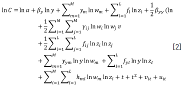
Where C is total cost, y is the output vector, w is the input prices vector and z is the environmental variables vector, t is a time trend, and vit and uit composed jointly the error term already defined. If it were not interactions between outputs and input prices, outputs and environmental variables, input prices and environmental variables, nor squared effects, the formula converges to a Cobb-Douglas form4.
4. Data and models
In this section, we first describe the database, defining variables, presenting its descriptive statistic, and thus we present the model to be estimated.
4.1. Data
The database was built with data provided by BCBA’s Offices of Planning and Control, and Economic Studies. Data comprise information from 01/2014 to 12/2016 for 58 branches (see Figure 1). The database is one balanced panel of 36 monthly observations for each branch (2,088 observations).
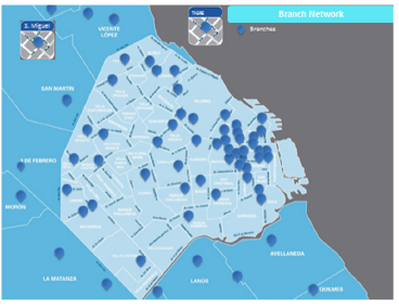
Figure 1 Map of Branches in the City of Buenos Aires and Surroundings
Table 2 describes the costs, outputs, inputs, input prices, time trend (to account- for seasonality), and environmental variables. We followed the literature consensus on variables to be included with the specificities of the case under study. All monetary variables were expressed in December 2016 prices, using as deflator the Construction Cost Index (ICC) estimated by the national statistics bureau (Instituto Nacional de Estadísticas y Censos, INDEC). Costs comprise labor, other administrative and loanable funds components. Outputs considered are number of loans and number of cashier operations (transactions).
Table 2 Variable definition
| Variable | Abridged name | Type | Definition | Variable in the cost frontier estimate |
|---|---|---|---|---|
| Total Costs | C | Cost | C = Labor Costs + Other Administrative Costs + Funding Costs = Salaries, wages and management remunerations plus social contributions + Non-labor, non-interests’ expenses + Interests paid for deposits | lc= log(C/W3) |
| Number of loans | Y2 | Output | Units | Ly2 = log(Y2) |
| Number of cashier operations | Y6 | Output | Units | Ly6 = log(Y6) |
| Staff | X1 | Input | Personnel at the Branch, proxy for labor input | |
| Size | X2 | Input | Size of the Branch (in M2 of surface), proxy for capital input | |
| Funding | X3 | Input | Time deposits stocks, proxy for loanable funds. | |
| Unit Labor Costs | W1 | Input Price | W1=C1/X1 | lw1=log(W1/W3) |
| Unit Administrative Costs | W2 | Input Price | W2=C2/X2 | lw2=log(W2/W3) |
| Unit Financial Costs | W3 | Input Price | W3=C3/X3 | numeraire |
| Time Trend | T | Trend | T=1, 2, … , N, for the initial (1) and final (N) month of the sample | T |
| EMAE | E | Environmental | Activity Index of Economic Performance in each place where the branch is working | E |
| Ratio of Automatization | RA | Environmental | Density of Automatic Terminals per non-commercial employee of the branch. | RA |
Source: own elaboration.
The inputs are labor (personnel), capital (proxied as the surface in m2 of each branch) and loanable funds. The input prices are the unit costs of labor, capital and loanable funds, the latter acting as the numeraire. A time trend and its square, because the model is a translog, were introduced, and two environmental variables were built to account for, the degree of automatization of the branch, and a monthly lead production indicator to account for the state of the economic cycle.
In the estimates, all cost, output and input prices variables are expressed in logarithms. The estimated cost functions are non-decreasing, linearly homogeneous and concave in the inputs if the β estimated with respect to outputs and input prices (first order coefficients) are not negative and satisfy the constraint that the sum of the β equals 1 for all considered inputs. If we divide the input price by any of them, the preceding conditions are satisfied. Our numeraire is W3, the loanable funds price.
Table 3 shows the descriptive statistics of the sample, where the values are in levels. For the sake of clarification, they are presented by group (outputs, inputs, input prices, and environmental).
Table 3 Descriptive Statistics of the sample
| Variable | Unit | Obs. | Mean | Standard Deviation | Minimum | Maximum |
|---|---|---|---|---|---|---|
| Costs | ||||||
| C | $ 2016 | 2,088 | 4,065,409 | 2,726,702 | 859,363 | 19,800,000 |
| Outputs | ||||||
| Y2 | Number of loans | 2.088 | 83.4224 | 78.3290 | 7 | 752 |
| Y6 | Number of cashier operations | 2.088 | 7487.8360 | 5773.224 | 868 | 44262 |
| Inputs | ||||||
| X1 | Employees (Total) | 2.088 | 19.0076 | 9.0497 | 9 | 79 |
| X2 | M2 | 2.088 | 1236.931 | 1935.148 | 105 | 10870 |
| X3 | Million 2016 AR$ | 2.088 | 3.1269 | 1.1688 | 1 | 14 |
| Input Prices | ||||||
| W1 | AR $ 2016 per Person | 2.088 | 1,145.229 | 439.8186 | 27 | 2,552 |
| W2 | AR $ 2016 per M2 | 2.088 | 121,023.3 | 274,699.4 | 4,912 | 2,856,964 |
| W3 | AR $ 2016 per unit of Funding | 2.088 | 0.0160 | 0.0053 | 0.004 | 0.0277 |
| Environmental | ||||||
| RA | Ratio (Automatic Self Service Terminals / Non-Commercial Employees) | 2.088 | 0.4770 | 0.0645 | 0.3100 | 0.7000 |
| EMAE | Index of Economic Activity | 2.088 | 146.1667 | 9.0345 | 132 | 170 |
Source: own elaboration base on BCBA and Dirección General de Estadísticas y Censos (DGEyC) data.
4.2 Models
We estimate two translog variants of stochastic cost frontiers such as formula [2], using two outputs (y2 and y6), and considering both cases, with and without environmental variables. We also estimate the Cobb-Douglas functional form as a restricted version of the translog (by eliminating from formula [2] quadratic and interaction terms). Using a Likelihood Ratio (LR) test between specifications we contrast the hypothesis of restrictions validity. We assume that efficiency remains constant over time (time invariant -TI-inefficiency term) due to the short and homogeneous period considered. It is expected marginal costs being positive on outputs, negative on input prices and positive on both three environmental variables. The sign of the interactions depends in each case on the relationship between the variables.
According to Coelli, Perelman and Romano (1999), frontier analysis presupposes all decision units share the same technology and environmental conditions. When the latter differs, there are two ways to consider their influence on efficiency: including the environmental variables as regressors (since it is supposed that environmental factors influence the shape of technology) or model the environmental factors as influencing directly the inefficiency term (since it is supposed that environmental factors do not influence the shape of technology, as in Battese and Coelli, 1995). The authors suggest that both approaches seem reasonable depending on the analyst’s philosophical perspective. The first approach produces efficiency scores which are the net of environmental influences (Coelli et al., 1999). Battese and Coelli (1995) provide a method to make compatible net and gross measures of inefficiency. The net efficiency, if all environmental characteristics are accounted for, can be interpreted as a measure of managerial performance.
5. Results
Table 4 presents the results for the estimated models. Translog models in both cases (with and without environmental variables) are preferred to Cobb-Douglas specifications according to the LR test. In the latter, both prices and outputs of the cost frontiers are significant. In the former, the linear terms for input prices are not significant, but square and interaction terms are significant in the translog with environmental variables and with a positive sign. Both linear coefficients for outputs are significant in the four specifications (with the exception of y6 in the translog without environmental variables). The negative sign for the linear coefficient of y2 is challenging; nevertheless, the full partial derivative of lnC with respect to y2 includes the quadratic and the interaction terms. Since environmental variables are significant, and the results of LR tests inform the same, the preferred specification is Model 1.
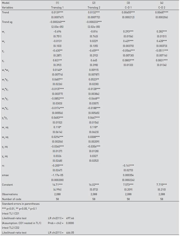
Table 5 presents the descriptive statistics of the efficiency results in each model.
Table 5 Cost efficiency scores in each model - descriptive statistic
| Model | Observations | Mean | Standard Deviation | Minimum | Maximum |
|---|---|---|---|---|---|
| Cost Efficiency TL1 | 2088 | 0,3308 | 0,1933 | 0,0248 | 0,9777 |
| Cost Efficiency TL2 | 2088 | 0,3516 | 0,2042 | 0,0255 | 0,9791 |
| Cost Efficiency CD 1 | 2088 | 0,3188 | 0,1960 | 0,0213 | 0,9761 |
| Cost Efficiency CD 2 | 2088 | 0,3330 | 0,2044 | 0,0219 | 0,9771 |
Source: own elaboration.
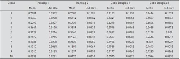
Table 6 presents the average efficiency of each decile of branches and its standard deviation according to each model. In this case, we can see that the first decile of branches in the selected model 1, achieves average values of 0.72 with a standard deviation of 0.13, while the tenth decile in the sample has average levels of 0.07 on average with a standard deviation of 0.03.
6. Discussion of results
As stated in the literature review, previous work has addressed different goals, such as rationalize the labor factor, reduce over-branching, manage seasonal ups and downs, compare between countries with different kind of banking development, evaluate size and performance, explore the waste of resources and its causes, and give the management tools for corporative control (see the different references there). Unlike those studies, and due to regulatory limits (for example to open or close branches), or because of agreements with the labor factor (treating the BCBA employees as public servants, and thus limiting the possibility of firing them), our goals are more modest: the bank is expanding its network, and we can contribute to the cost effectiveness of the new branches.
Based on the results of the cost efficiency models, we can formulate some implications for management. Let us suppose that the board of the bank wants to analyze which resources to devote to a new branch5.
Table 6 shows the mean and standard deviation of output in the best and worst deciles of branches under model 1. The bottom line of the table is the quotient between both means. First, the first decile branches are smaller in terms of labor and non-labor inputs, and also in loans and transactions’ production.
Table 7 also sheds light on the differences between cost efficient branches and inefficient ones. Cost-efficient branches have on average 12.5 employees, where 5.8 are commercial, while inefficient ones have 38 with 17 commercial. The space devoted to the most efficient branches is sensibly smaller than those in inefficient ones. The impact of costs here is the way they are imputed: since all non-labor, non-funding costs are attributed to square meters of surface (because some physical unit of “capital” factor is necessary), the biggest branches are costly.
Table 7 Average mean and standard deviation of outputs mixes, output and environmental variables in most efficient and least efficient deciles (Translog 1)
| X1 | Commercial staff | X2 | x1/x2 | ra | rb | rc | y2 | y6 | |
|---|---|---|---|---|---|---|---|---|---|
| First Decile Mean | 12.495 | 5.814 | 283.667 | 0.0565 | 0.0011 | 0.0292 | 0.365 | 50.07 | 4130.22 |
| First Decile Std. Dev. | 2.189 | 1.503 | 140.388 | 0.0339 | 0.0557 | 0.0155 | 0.155 | 18.37 | 1157.10 |
| Tenth Decile Mean | 38.094 | 17.350 | 5676.800 | 0.0144 | 0.0007 | 0.0182 | 0.244 | 224.53 | 19646.22 |
| Tenth Decile Std. Dev | 18.965 | 8.433 | 4231.094 | 0.0157 | 0.0426 | 0.0125 | 0.050 | 181.56 | 12150.22 |
| First Decile Mean/Tenth Decile Mean | 0.115 | 0.178 | 0.0050 | 3.9075 | 1.5795 | 1.6006 | 1.496 | 0.2230 | 0.2102 |
Source: own elaboration.
The differences also appear in the input mix: the most efficient branches have an intensity of personnel per square meter which is 3.92 times greater, and a productivity of both factors is lower in the efficient branches. The physical productivity of large branches is greater, nevertheless with high costs. The level of automatization (ra) is not the same in both sets of branches, and there are differences in the business clients on total customer ratio (rb with respect to the value of the least efficient in the most efficient decile) and in the proportion of commercial to total personnel (rc). Note that rb and rc did not prove significant in the estimates and were eliminated in the final models presented in Table 4.
In sum, as a managerial implication, if the bank under analysis wants to open a new branch with the characteristics of the best performing of the existent ones, it should have 12 employees, 47% of whom are commercial, counted with a surface of 283 square meters, and have at least 1 automatic service terminal (ra times the non-commercial staff). In addition, it should register at least 3% of commercial over total customers and follow the same pattern of output mix as the average branch.
7. Conclusions
This paper estimates cost efficiency frontiers at branch level for a three-year period using monthly data for the BCBA bank. We estimate two models with and without environmental variables, following translog and Cobb-Douglas specifications.
The average efficiency of the entire sample for the preferred models is in the line of 0.33, where the first decile of efficient branches averages 0.72 and the tenth decile of inefficient ones, averages only 0.07. This means that the set of more inefficient branches is one-tenth as efficient as the best situated.
The cost-efficient ones are smaller than the cost inefficient -both in personnel and in surface-, but more pronounced in the latter variable, our proxy for “capital” factor. Also, the proportion of commercial to total personnel is higher in the most efficient branches.
Sometimes, the managerial goals are set in terms of some output quantitative mix, irrespective of their costs. Should the output goal of the branches be changed, for example, by changing weights on each product, the cost efficiency ranking will also change. In the same vein, if central bank current regulations on branch creation and shutting were lifted, efficiency levels would be different. But, considering both, managerial and regulatory constraints as binding, one can use a minimalist approach of the study at least to improve efficiency in the margin: if the bank under analysis wants to open a new branch with the characteristics of the most cost efficient of the existent ones, it should have 12 employees, 46% of whom are commercial, counted with a surface of 283 square meters, and have at least 1 automatic service terminal. It should register at least 3% of total customers and follow the same pattern of output mix as the average branch.